Synthetic control with pymc models

import arviz as az

import causalpy as cp

%load_ext autoreload
%autoreload 2
%config InlineBackend.figure_format = 'retina'
seed = 42

Load data

df = cp.load_data("sc")
treatment_time = 70

Donor pool selection

Before fitting, it is good practice to inspect pairwise correlations among units in the pre-treatment period. Negatively correlated donors should be excluded to avoid interpolation bias [Abadie, 2021, Abadie et al., 2010].

pre = df.loc[:treatment_time]
corr, ax = cp.plot_correlations(pre, columns=["a", "b", "c", "d", "e", "f", "g"])
ax.set(title="Pre-treatment correlations")

[Text(0.5, 1.0, 'Pre-treatment correlations')]

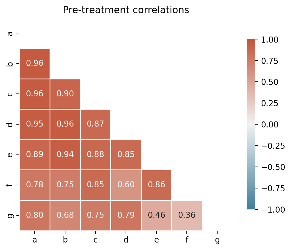
All control units are positively correlated with the treated unit (actual), so no donor pool curation is needed for this dataset. In practice, you would exclude any controls with negative or near-zero correlations.

Run the analysis

Note

The random_seed keyword argument for the PyMC sampler is not necessary. We use it here so that the results are reproducible.

Convex Hull Assumption

The synthetic control method uses non-negative weights that sum to one. This means the synthetic control is a convex combination of the control units—it can only produce values within the range spanned by the controls at each time point.

Note

For the method to work well, the treated unit’s pre-intervention trajectory should lie within the “envelope” of the control units. If all controls are consistently above or below the treated unit, the method cannot construct an accurate counterfactual.

CausalPy automatically checks this assumption when you create a SyntheticControl object and will issue a warning if violated. See the Convex hull condition glossary entry and Abadie et al. [2010] for more details. The Augmented Synthetic Control Method [Ben-Michael et al., 2021] can handle cases where this assumption is violated.

df.head()

	a	b	c	d	e	f	g	counterfactual	causal effect	actual
0	0.806091	-0.271100	0.664254	1.705922	-1.449230	0.785439	-1.234083	-0.232966	-0.0	-0.076404
1	1.442677	0.462594	0.559940	1.862041	-1.615366	0.386238	-1.798470	-0.069413	-0.0	-0.063946
2	1.916486	0.845719	0.894046	2.061073	-1.978696	0.971803	-0.490287	0.095440	-0.0	0.392813
3	2.001511	1.067162	0.288606	1.934534	-2.093951	1.889334	-0.478545	0.261716	-0.0	0.133106
4	2.662849	1.243252	0.966345	2.482698	-1.407598	2.184504	-0.434592	0.429432	-0.0	0.293294

result = cp.SyntheticControl(
    df,
    treatment_time,
    control_units=["a", "b", "c", "d", "e", "f", "g"],
    treated_units=["actual"],
    model=cp.pymc_models.WeightedSumFitter(
        sample_kwargs={"target_accept": 0.95, "random_seed": seed}
    ),
)

Show code cell output Hide code cell output

Initializing NUTS using jitter+adapt_diag...

Multiprocess sampling (4 chains in 4 jobs)

NUTS: [beta, y_hat_sigma]

Sampling 4 chains for 1_000 tune and 1_000 draw iterations (4_000 + 4_000 draws total) took 14 seconds.

Sampling: [beta, y_hat, y_hat_sigma]

Sampling: [y_hat]

Sampling: [y_hat]

Sampling: [y_hat]

Sampling: [y_hat]

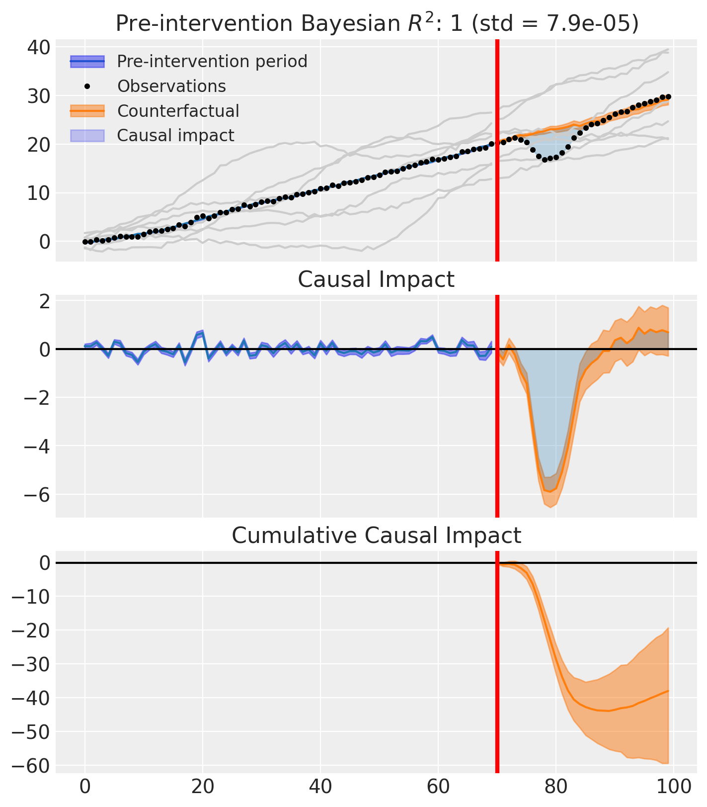
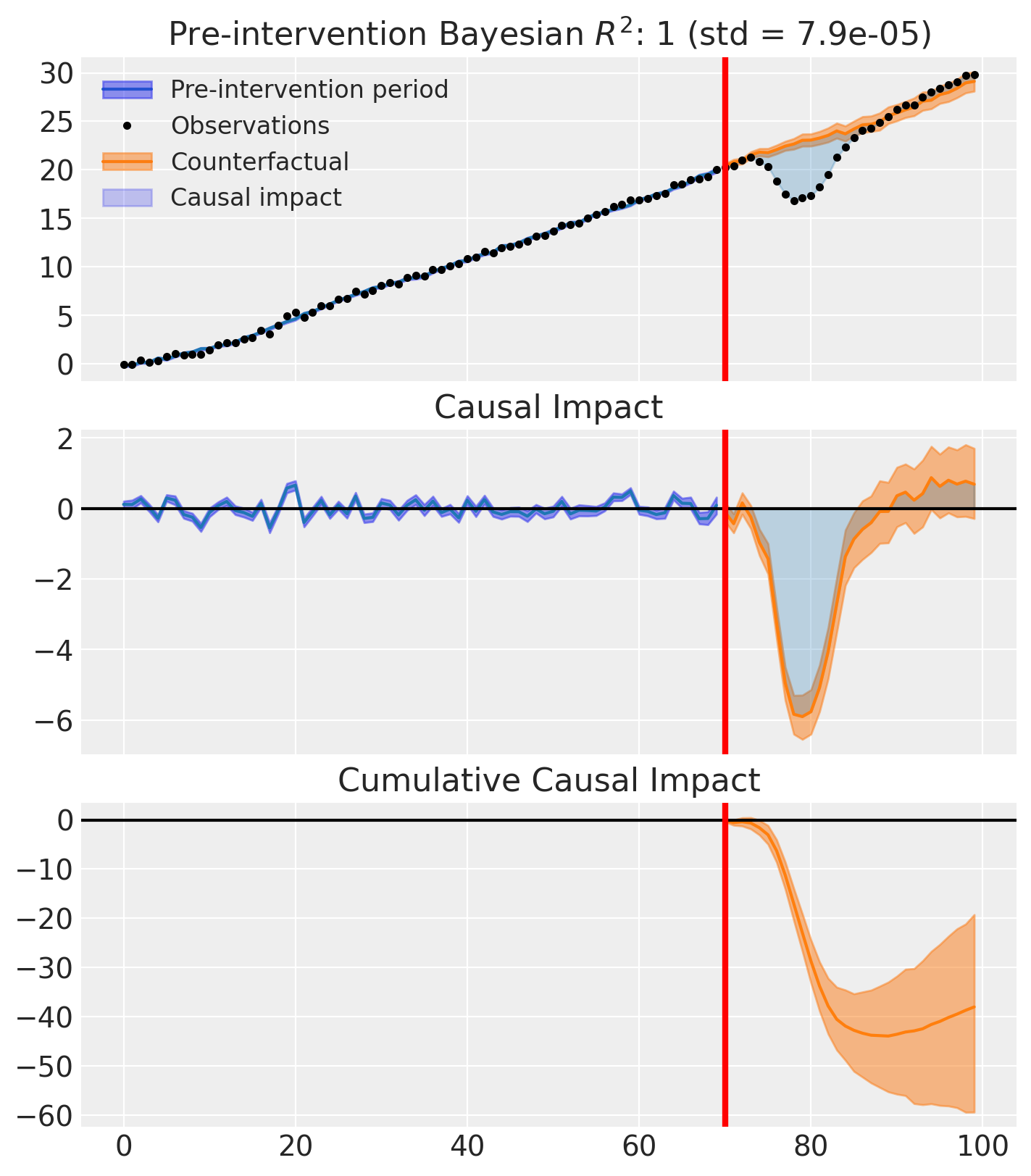
fig, ax = result.plot(plot_predictors=True)

result.summary()

================================SyntheticControl================================
Control units: ['a', 'b', 'c', 'd', 'e', 'f', 'g']
Treated unit: actual
Model coefficients:
    a            0.056, 94% HDI [0.0031, 0.14]
    b            0.2, 94% HDI [0.14, 0.25]
    c            0.21, 94% HDI [0.13, 0.29]
    d            0.058, 94% HDI [0.0061, 0.12]
    e            0.26, 94% HDI [0.23, 0.29]
    f            0.11, 94% HDI [0.068, 0.15]
    g            0.11, 94% HDI [0.074, 0.15]
    y_hat_sigma  0.25, 94% HDI [0.21, 0.3]
Pre-treatment correlation (actual): 0.9992

We can get nicely formatted tables from our integration with the maketables package.

from maketables import ETable

result.set_maketables_options(hdi_prob=0.95)
ETable(result, coef_fmt="b:.3f \n [ci95l:.3f, ci95u:.3f]")

	y
	(1)
coef
a	0.056 [0.000, 0.126]
b	0.195 [0.142, 0.252]
c	0.213 [0.130, 0.292]
d	0.058 [0.001, 0.116]
e	0.256 [0.224, 0.290]
f	0.110 [0.067, 0.152]
g	0.112 [0.073, 0.151]
stats
N	100
Bayesian R2	0.998
Format of coefficient cell: Coefficient [95% CI Lower, 95% CI Upper]

As well as the model coefficients, we might be interested in the average causal impact and average cumulative causal impact.

az.summary(result.post_impact.mean("obs_ind"))

	mean	sd	hdi_3%	hdi_97%	mcse_mean	mcse_sd	ess_bulk	ess_tail	r_hat
x[actual]	-1.267	0.367	-1.979	-0.641	0.014	0.007	731.0	1495.0	1.01

Warning

Care must be taken with the mean impact statistic. It only makes sense to use this statistic if it looks like the intervention had a lasting (and roughly constant) effect on the outcome variable. If the effect is transient, then clearly there will be a lot of post-intervention period where the impact of the intervention has ‘worn off’. If so, then it will be hard to interpret the mean impacts real meaning.

We can also ask for the summary statistics of the cumulative causal impact.

# get index of the final time point
index = result.post_impact_cumulative.obs_ind.max()
# grab the posterior distribution of the cumulative impact at this final time point
last_cumulative_estimate = result.post_impact_cumulative.sel({"obs_ind": index})
# get summary stats
az.summary(last_cumulative_estimate)

	mean	sd	hdi_3%	hdi_97%	mcse_mean	mcse_sd	ess_bulk	ess_tail	r_hat
x[actual]	-38.005	11.019	-59.384	-19.237	0.407	0.211	731.0	1495.0	1.01

Effect Summary Reporting

For decision-making, you often need a concise summary of the causal effect with key statistics. The effect_summary() method provides a decision-ready report with average and cumulative effects, HDI intervals, tail probabilities, and relative effects.

# Generate effect summary for the full post-period
stats = result.effect_summary(treated_unit="actual")
stats.table

	mean	median	hdi_lower	hdi_upper	p_gt_0	relative_mean	relative_hdi_lower	relative_hdi_upper
average	-1.266830	-1.269718	-2.001737	-0.613731	0.00075	-5.155195	-7.941135	-2.576623
cumulative	-38.004895	-38.091551	-60.052099	-18.411916	0.00075	-5.155195	-7.941135	-2.576623

print(stats.text)

During the Post-period (70 to 99), the response variable had an average value of approx. 23.21. By contrast, in the absence of an intervention, we would have expected an average response of 24.47. The 95% interval of this counterfactual prediction is [23.82, 25.21]. Subtracting this prediction from the observed response yields an estimate of the causal effect the intervention had on the response variable. This effect is -1.27 with a 95% interval of [-2.00, -0.61].

Summing up the individual data points during the Post-period, the response variable had an overall value of 696.16. By contrast, had the intervention not taken place, we would have expected a sum of 734.17. The 95% interval of this prediction is [714.58, 756.22].

The 95% HDI of the effect [-2.00, -0.61] does not include zero. The posterior probability of a decrease is 0.999. Relative to the counterfactual, the effect represents a -5.16% change (95% HDI [-7.94%, -2.58%]).

This analysis assumes that the control units used to construct the synthetic counterfactual were not themselves affected by the intervention, and that the pre-treatment relationship between control and treated units remains stable throughout the post-treatment period. We recommend inspecting model fit, examining pre-intervention trends, and conducting sensitivity analyses (e.g., placebo tests) to support any causal conclusions drawn from this analysis.

You can customize the summary in several ways:

• Window: Analyze a specific time period instead of the full post-period

• Direction: Specify whether you’re testing for an increase, decrease, or two-sided effect

• Options: Include/exclude cumulative or relative effects

# Example: Analyze first half of post-period
post_indices = result.datapost.index
window_start = post_indices[0]
window_end = post_indices[len(post_indices) // 2]

stats_windowed = result.effect_summary(
    window=(window_start, window_end),
    treated_unit="actual",
    direction="two-sided",
    cumulative=True,
    relative=True,
)

stats_windowed.table

	mean	median	hdi_lower	hdi_upper	p_two_sided	prob_of_effect	relative_mean	relative_hdi_lower	relative_hdi_upper
average	-2.672167	-2.655041	-3.192889	-2.168353	0.0	1.0	-11.888489	-13.89799	-9.878958
cumulative	-42.754673	-42.480652	-51.086217	-34.693647	0.0	1.0	-11.888489	-13.89799	-9.878958

print(stats_windowed.text)

During the Post-period (70 to 85), the response variable had an average value of approx. 19.78. By contrast, in the absence of an intervention, we would have expected an average response of 22.45. The 95% interval of this counterfactual prediction is [21.95, 22.97]. Subtracting this prediction from the observed response yields an estimate of the causal effect the intervention had on the response variable. This effect is -2.67 with a 95% interval of [-3.19, -2.17].

Summing up the individual data points during the Post-period, the response variable had an overall value of 316.49. By contrast, had the intervention not taken place, we would have expected a sum of 359.25. The 95% interval of this prediction is [351.19, 367.58].

The 95% HDI of the effect [-3.19, -2.17] does not include zero. The posterior probability of an effect is 1.000. Relative to the counterfactual, the effect represents a -11.89% change (95% HDI [-13.90%, -9.88%]).

This analysis assumes that the control units used to construct the synthetic counterfactual were not themselves affected by the intervention, and that the pre-treatment relationship between control and treated units remains stable throughout the post-treatment period. We recommend inspecting model fit, examining pre-intervention trends, and conducting sensitivity analyses (e.g., placebo tests) to support any causal conclusions drawn from this analysis.

Sensitivity analysis

This section walks through placebo-in-time diagnostics for synthetic control using the pipeline API (EstimateEffect → SensitivityAnalysis → GenerateReport). For the shared workflow concepts — Pipeline, pluggable checks, and HTML reports — see Pipeline Workflow. For the full menu of checks and how they relate, see Sensitivity Checks in Pipeline Workflows.

Related checks for synthetic control

Several pipeline checks are designed for Synthetic Control designs, each targeting a different vulnerability:

• PlaceboInTime (default; covered below) — shifts the treatment time backward into the pre-treatment period and asks whether pseudo-interventions produce effects comparable to the real one. Requires a PyMC-backed model.

• ConvexHullCheck — verifies that pre-treatment treated values lie within the range spanned by the donor pool. A failure indicates the synthetic control fit relies on extrapolation rather than interpolation.

• LeaveOneOut — drops each donor unit in turn and refits, surfacing donors that exert disproportionate influence on the estimate.

• PlaceboInSpace — relabels each control unit as if it were treated and compares the resulting placebo effects to the actual treated effect [Abadie et al., 2010]. If many controls produce effects as large as the treated unit, the original estimate is less distinctive.

• PriorSensitivity — a cross-cutting Bayesian check: re-fits the same specification under alternative priors and compares effect summaries. Useful for diagnosing prior-data conflict.

Other checks (e.g. PreTreatmentPlaceboCheck, BandwidthSensitivity, McCraryDensityTest) target different estimators and are not applicable here.

Placebo-in-time check

PlaceboInTime is the synthetic control default check registered in cp.SensitivityAnalysis.default_for(cp.SyntheticControl). It answers a falsification question central to synthetic control practice: if we pretended the intervention happened earlier, would we still see an effect? Placebo and falsification exercises are a standard component of synthetic-control credibility [Abadie, 2021].

How it works. The check shifts the treatment time backward into the pre-intervention period, fitting n_folds placebo experiments. From each fold it extracts the posterior cumulative impact, then fits a hierarchical Bayesian status-quo model that pools across folds to characterise the distribution of effects when no real intervention occurred. The actual cumulative impact is compared against this learned null, and the check passes when the posterior probability that the real effect lies outside the null distribution exceeds threshold (default 0.95). PlaceboInTime requires a PyMC model because it consumes posterior draws.

Walkthrough

1. Fit the synthetic control as above so the experiment exposes a treatment_time and post_impact.

2. Run the pipeline cell below. EstimateEffect re-fits the experiment inside the pipeline so PlaceboInTime can clone the configuration for each placebo fold.

3. Inspect the printed CheckResult.text for the verdict and per-fold summaries; the full hierarchical-null draws are available in metadata["null_samples"].

4. Open the HTML report (iframe) for a consolidated view alongside the main estimates.

Interpreting the result on this dataset. On the example dataset above the verdict sits right on the 0.95 threshold — the printed P(actual outside null) lands near 0.92, and small MCMC sampling noise can push it either side of the cutoff between runs (see the reproducibility note below). Read the verdict as borderline rather than as a clean pass or fail. The actual cumulative impact (≈ −38) is clearly large, but the hierarchical null inferred from the placebo folds is wide enough that the check cannot discriminate sharply on this data. Drilling into the per-fold summaries explains why: fold 1’s pseudo-treatment time lands at index 12, leaving only 12 pre-treatment observations to fit a synthetic control on 7 donors. That model is poorly identified, so its posterior cumulative impact carries a large standard deviation, which inflates tau in the hierarchical status-quo model and broadens the null distribution. Fold 2, with a 41-row pre-period, behaves much better.

Treat this as an illustrative borderline case rather than a substantive verdict on the headline causal estimate — with only n_folds=2 on a short series, this dataset does not give the placebo-in-time check enough independent evidence to call it either way. In general, a pass means the actual cumulative impact is unlikely under the status-quo null inferred from placebo folds — consistent with a real treatment effect. A fail means the placebo folds produced effects of similar magnitude, so the real effect is hard to distinguish from background variability. Like any single diagnostic, this is necessary but not sufficient: passing does not prove identification, and failing does not prove the absence of an effect [Reichardt, 2019].

Note

Known limitations being tracked. Two upstream issues affect how this check behaves on the example data above. Until both are resolved, treat borderline P(actual outside null) values on this dataset as exactly that — borderline — rather than as evidence for or against the headline estimate.

• Placebo windows that land too early (#875): PlaceboInTime derives intervention_length from data.index.max() - treatment_time and shifts the placebo treatment time backward by multiples of that length. When the resulting earliest fold has a short pre-period (as fold 1 does here), the synthetic control fit on that fold is noisy and can dominate the hierarchical null. The proposed fix lets users pass an explicit intervention_length and adds a configurable minimum pre-period per fold so weak folds can be skipped. As an interim workaround you can pass an experiment_factory to PlaceboInTime that fits placebo folds on a smaller donor pool or a shorter intervention window.

• Reproducibility gap in the internal posterior predictive (#876): even with random_seed plumbed through both sample_kwargs and the constructor, the internal pm.sample_posterior_predictive call for theta_new is not currently seeded, so the printed P(actual outside null) can drift by ~0.01–0.02 between runs and may straddle the 0.95 threshold. The proposed fix unifies the seed surface so the constructor’s random_seed deterministically governs every stochastic stage of the check.

If this check fails

A failing PlaceboInTime indicates that pseudo-interventions in the pre-period produced effects comparable to the real one — or, as on the dataset above, that the inferred null is too wide to rule them out. Concrete steps to diagnose and address this:

1. Inspect fold summaries. The metadata["fold_results"] field on the CheckResult lists each placebo fold’s posterior mean and standard deviation. A single fold with an outsized sd (as fold 1 has here) is usually a sign that its pre-period is too short to identify the synthetic control fit, rather than evidence against the headline causal estimate.

2. Reconsider the donor pool. Highly correlated donors stabilise the synthetic control; donors whose pre-treatment correlation with the treated unit is weak — or unstable across windows — can introduce noise that shows up as spurious placebo effects. Re-run the pre-treatment correlation diagnostic above and prune the pool accordingly [Abadie, 2021].

3. Add complementary SC-specific checks. Run LeaveOneOut to see whether any single donor drives the result, and PlaceboInSpace to check whether spurious effects are common across control units. Persistent failures across multiple diagnostics are a stronger signal than any one alone.

4. Sanity-check the convex-hull condition. Use ConvexHullCheck to verify the treated unit’s pre-period trajectory lies within the support of the donor pool. Outside-the-hull fits depend on extrapolation and are more vulnerable to false positives [Abadie et al., 2010].

5. Probe prior sensitivity. Re-fit with cp.checks.PriorSensitivity using tighter or more diffuse priors. If the conclusion flips, prior-data conflict is contributing to the fragile inference.

sensitivity_result = cp.Pipeline(
    data=df,
    steps=[
        cp.EstimateEffect(
            method=cp.SyntheticControl,
            treatment_time=treatment_time,
            control_units=["a", "b", "c", "d", "e", "f", "g"],
            treated_units=["actual"],
            model=cp.pymc_models.WeightedSumFitter(
                sample_kwargs={"target_accept": 0.95, "random_seed": seed},
            ),
        ),
        cp.SensitivityAnalysis(
            checks=[
                cp.checks.PlaceboInTime(
                    n_folds=2,
                    sample_kwargs={"random_seed": seed, "progressbar": False},
                    random_seed=seed,
                )
            ],
        ),
        cp.GenerateReport(include_plots=True),
    ],
).run()

for cr in sensitivity_result.sensitivity_results:
    print(cr.text)

Initializing NUTS using jitter+adapt_diag...

Multiprocess sampling (4 chains in 4 jobs)

NUTS: [beta, y_hat_sigma]

Sampling 4 chains for 1_000 tune and 1_000 draw iterations (4_000 + 4_000 draws total) took 14 seconds.

Sampling: [beta, y_hat, y_hat_sigma]

Sampling: [y_hat]

Sampling: [y_hat]

Sampling: [y_hat]

Sampling: [y_hat]

Initializing NUTS using jitter+adapt_diag...

Multiprocess sampling (4 chains in 4 jobs)

NUTS: [beta, y_hat_sigma]

Sampling 4 chains for 1_000 tune and 1_000 draw iterations (4_000 + 4_000 draws total) took 4 seconds.

Sampling: [beta, y_hat, y_hat_sigma]

Sampling: [y_hat]

Sampling: [y_hat]

Sampling: [y_hat]

Sampling: [y_hat]

/Users/benjamv/git/CausalPy/causalpy/experiments/synthetic_control.py:118: UserWarning: Control units ['g' (r=-0.544)] have pre-treatment correlation below 0.0 or undefined with treated unit 'actual'. Consider excluding them from the donor pool. Use cp.plot_correlations() to inspect. See Abadie (2021) for guidance on donor pool selection.
  self._check_donor_correlations()

Initializing NUTS using jitter+adapt_diag...

Multiprocess sampling (4 chains in 4 jobs)

NUTS: [beta, y_hat_sigma]

Sampling 4 chains for 1_000 tune and 1_000 draw iterations (4_000 + 4_000 draws total) took 10 seconds.

Sampling: [beta, y_hat, y_hat_sigma]

Sampling: [y_hat]

Sampling: [y_hat]

Sampling: [y_hat]

Sampling: [y_hat]

Initializing NUTS using jitter+adapt_diag...

Multiprocess sampling (4 chains in 4 jobs)

NUTS: [mu_status_quo, tau_status_quo, fold_z]

Sampling 4 chains for 1_000 tune and 1_000 draw iterations (4_000 + 4_000 draws total) took 1 seconds.

Sampling: [theta_new]

Placebo-in-time analysis: 2 of 2 folds completed.
Hierarchical status-quo model: mu=2.27, tau=12.75.
Actual cumulative impact: -38.00. P(actual outside null) = 0.923.
NOT SUPPORTED — actual effect is within the null distribution.
Fold 1: pseudo treatment at 12 — mean=16.71, sd=30.53
Fold 2: pseudo treatment at 41 — mean=-1.81, sd=9.18

import html as html_module
import warnings

from IPython.display import HTML

with warnings.catch_warnings():
    warnings.filterwarnings(
        "ignore", "Consider using IPython.display.IFrame", UserWarning
    )
    display(
        HTML(
            f'<iframe srcdoc="{html_module.escape(sensitivity_result.report)}" '
            f'width="100%" height="600" style="border:1px solid #ccc;"></iframe>'
        )
    )